Both the volume and variety of data available to geophysicists, along with computational techniques and resources to process them, continue to grow rapidly. For many users, there is a corresponding increase in the burden of “data management” including collection and preparation for processing. Furthermore, data are often organized to support discovery and access for specific workflows.

In this How-To article, we will demonstrate how you can use the popular ObsPy Python framework to catalog large data sets and efficiently access subsets for general use, and with relatively little code. Specifically, we illustrate the use of OsbPy’s TSIndex module to significantly reduce the burden of organizing miniSEED data while supporting efficient, arbitrary access.

Our test data set is continuous data for the month of January 2008 from the USArray Transportable Array totaling over 90 gigabytes. The data were written to local storage with all channels for a given station and day in the same file, for a total of over 11,000 files. These data were downloaded using IRIS’s ROVER tool, which is highly recommended for collecting large data sets. The ROVER tool also generates the data catalog (aka index) while downloading data, making the data immediately ready to use with TSIndex module.

It is important to emphasize that the volume of data and how it is stored on disk is (mostly) unimportant. The same approach described has been used for data sets of 40+ terabytes, and it could have all been in a single file (within storage system limits). This is, in fact, the point of using the TSIndex module, discovery and reading of data is (mostly) independent of the data storage strategy.

ObsPy version 1.3 was used for the following work and is highly recommended if you will use the capabilities illustrated.

Indexing a miniSEED data set

Note If the ROVER tool was used to collect the data this index has already been generated, and this step can be skipped.

The first step after collecting the data is to build the index, which is a catalog of the data, stored in an SQLite database. Indexing capability is included in ObsPy and is recommended, even though the index could be built manually using the mseedindex program.

In this test case all miniSEED files are stored in a data directory under the current working directory. The index is generated with the following code:

>>> from obspy.clients.filesystem.tsindex import Indexer
>>> indexer = Indexer('data')
>>> indexer.run()

The name of the resulting index database, unless otherwise configured, is timeseries.sqlite and now we have this:

% ls -l
total 82072
drwxr-xr-x  3 chad  group        96 May  3 16:36 data
-rw-r--r--  1 chad  group  41123840 May  3 16:40 timeseries.sqlite

The timeseries.sqlite file is an SQLite3 database and may be accessed as such for any purpose. The schema is documented.

Reading miniSEED data using the index

With an index, ObsPy can now read arbitrary selections of data from this set very efficiently. The TSIndex module implements the Client interface that is common for data sources in ObsPy. Initializing the read capability is as simple as:

>>> from obspy.clients.filesystem.tsindex import Client
>>> client = Client('timeseries.sqlite')

With that you can query the “client” for data availability. Continuous traces can be queried using the get_availability method, and extents, i.e. earliest and latest times, can be queried using the get_availability_extent method. For example, to find the extents of the TA stations whose codes begin with “B1”:

>>> extents = client.get_availability_extent(network="TA", station="B1*")
>>> for extent in extents:
...     print("{0:<3} {1:<6} {2:<3} {3:<4} {4} {5}".format(*extent))

TA  B10A       BHE  2008-01-01T00:00:00.000000Z 2008-02-01T00:00:00.000000Z
TA  B10A       BHN  2008-01-01T00:00:00.000000Z 2008-02-01T00:00:00.000000Z
TA  B10A       BHZ  2008-01-01T00:00:00.000000Z 2008-02-01T00:00:00.000000Z
TA  B11A       BHE  2008-01-01T00:00:00.024998Z 2008-01-31T23:59:59.999998Z
TA  B11A       BHN  2008-01-01T00:00:00.024998Z 2008-01-31T23:59:59.999998Z
TA  B11A       BHZ  2008-01-01T00:00:00.024998Z 2008-01-31T23:59:59.999998Z
TA  B12A       BHE  2008-01-01T00:00:00.000000Z 2008-02-01T00:00:00.000000Z
TA  B12A       BHN  2008-01-01T00:00:00.000000Z 2008-02-01T00:00:00.000000Z
TA  B12A       BHZ  2008-01-01T00:00:00.000000Z 2008-02-01T00:00:00.000000Z
TA  B13A       BHE  2008-01-01T00:00:00.000000Z 2008-01-31T18:54:49.500000Z
TA  B13A       BHN  2008-01-01T00:00:00.000000Z 2008-01-31T18:54:49.500000Z
TA  B13A       BHZ  2008-01-01T00:00:00.000000Z 2008-01-31T18:54:49.500000Z
... more of that stuff ...

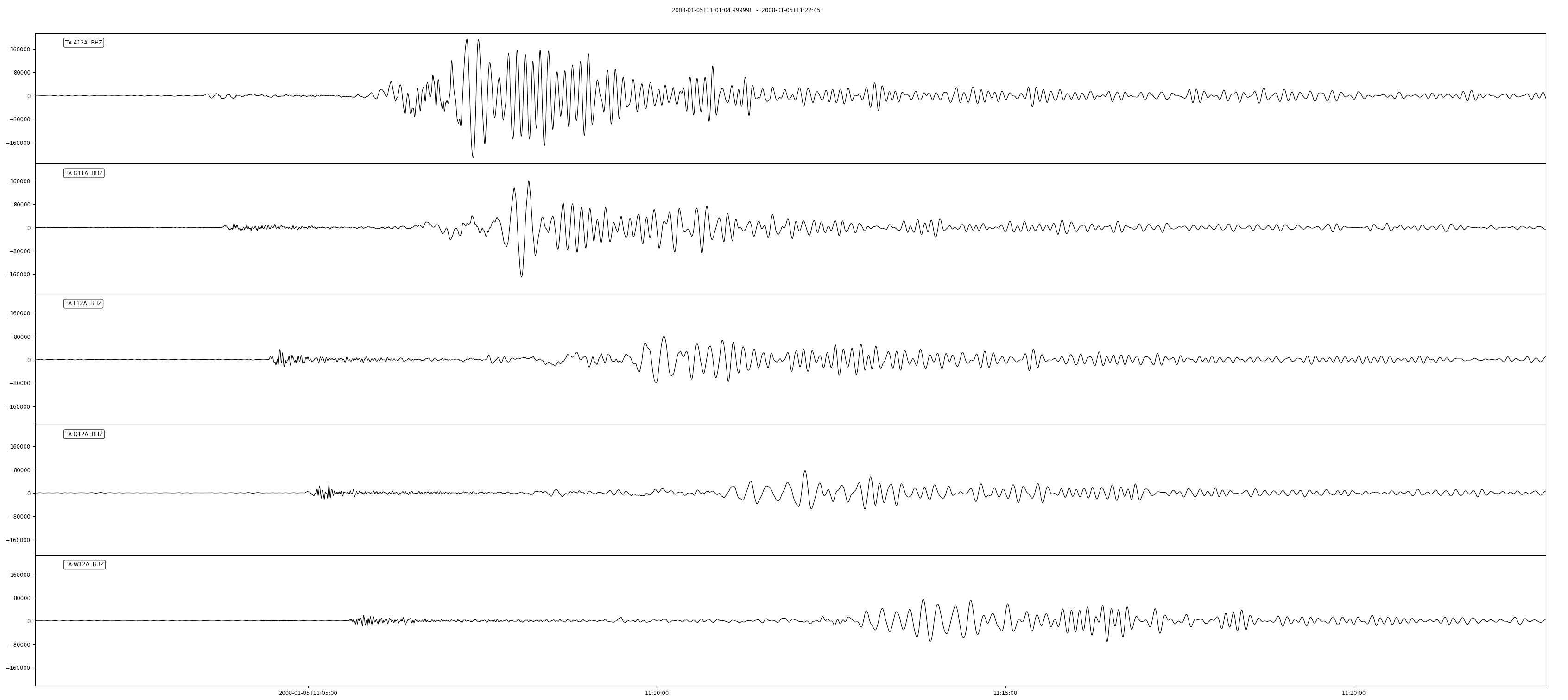
This data set includes signals for many events. If you wanted to focus on one of the bigger earthquakes (M6.5, Haida Gwaii, origin time: 2008-01-05T11:01:05.55Z) the data are easily read into memory and plotted:

>>> from obspy import UTCDateTime
>>> event_origin = UTCDateTime(2008, 1, 5, 11, 1, 5)

# Read a few selected channels for 1300 seconds from origin time and plot
>>> st = client.get_waveforms("TA", "A12A,G11A,L12A,Q12A,W12A", "*", "BHZ", event_origin, event_origin + 1300)
>>> st.plot()

Note that the data access only takes a few seconds and no knowledge of the data organization is needed.

Resulting figure:

Reading more than a few traces

In the following example we collect metadata for the TA stations (this could also be stored as a StationXML file locally, but we fetch from IRIS for convenience and illustration):

# Fetch station-level metadata
>>> from obspy.clients.fdsn import Client as MetaClient
>>> metaclient = MetaClient("IRIS")
>>> inventory = metaclient.get_stations(network="TA", channel="BH?", level="station",
...                                     starttime=event_origin,
...                                     endtime=event_origin + 1300)

We then read all BHZ channels for the same earthquake signal time window as before and populate the coordinates for each trace:

>>> st = client.get_waveforms("TA", "*", "*", "BHZ", event_origin, event_origin + 1300)

# Attach station-level coordinates to traces (good enough for a rough record section)
>>> from obspy.core import AttribDict
>>> for tr in st:
...    for station in inventory[0].stations:
...        if tr.stats.station == station.code:
...            tr.stats.coordinates = \
...                AttribDict(dict(latitude=station.latitude,
...                           longitude=station.longitude,
...                           elevation=station.elevation))

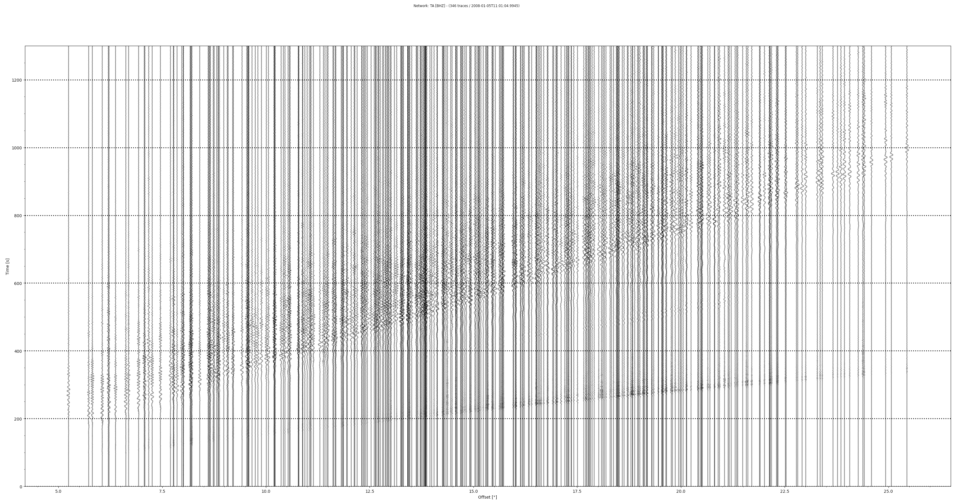
Finally we plot a full TA record section:

# Earthquake coordinates
>>> evlat = 51.2448
>>> evlon = -130.8641

>>> st.plot(type='section', dist_degree=True, ev_coord=(evlat, evlon), linewidth=2, grid_linewidth=2)

Resulting figure:

Summary and key points

The combination of an index for your miniSEED data and the TSIndex module in ObsPy allows you to efficiently read arbitrary selections from your local data set, without much care about how the data are organized in the storage system. Furthermore, miniSEED data from multiple sources (e.g. multiple data centers) can be combined in the same index and accessed seamlessly (they do not need to be stored in the same structure!).

Gotchas and footnotes

• In general the organization of miniSEED into files and directories does not matter. However, the indexing and read access will be less efficient if the data are not grouped by channel in the storage system. For example, if a file contains all the channels from a given station for a given time period, it is best if all the records for a given channel are in time order and grouped, i.e. sequential within the file.

• The indexing system is sensitive to leap seconds and may complain if a “leap second file” is not available. To address this edge case, you may wish to download the official leap second file to the working directory where you are building the index, e.g.:

% curl -JLO 'https://www.ietf.org/timezones/data/leap-seconds.list'