Summary
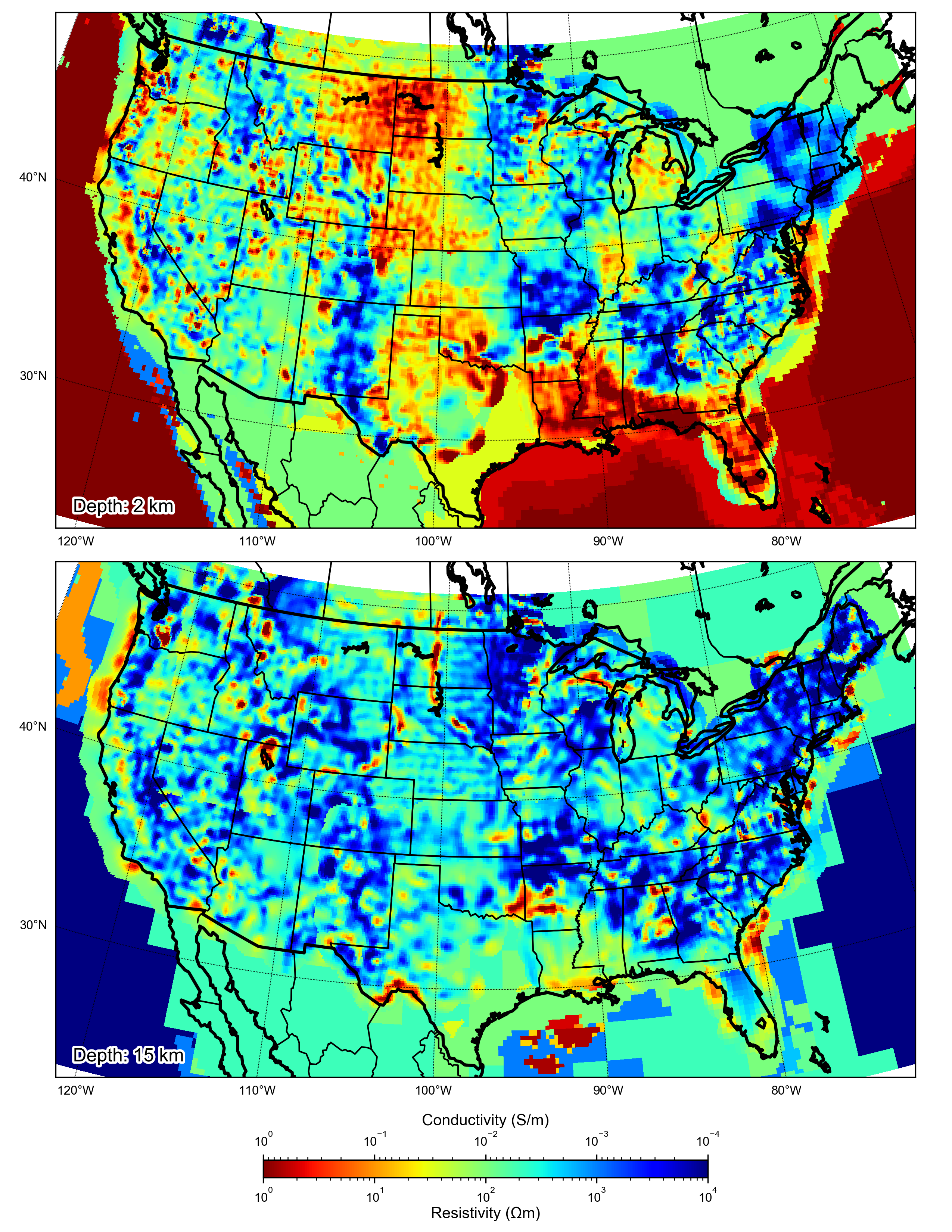
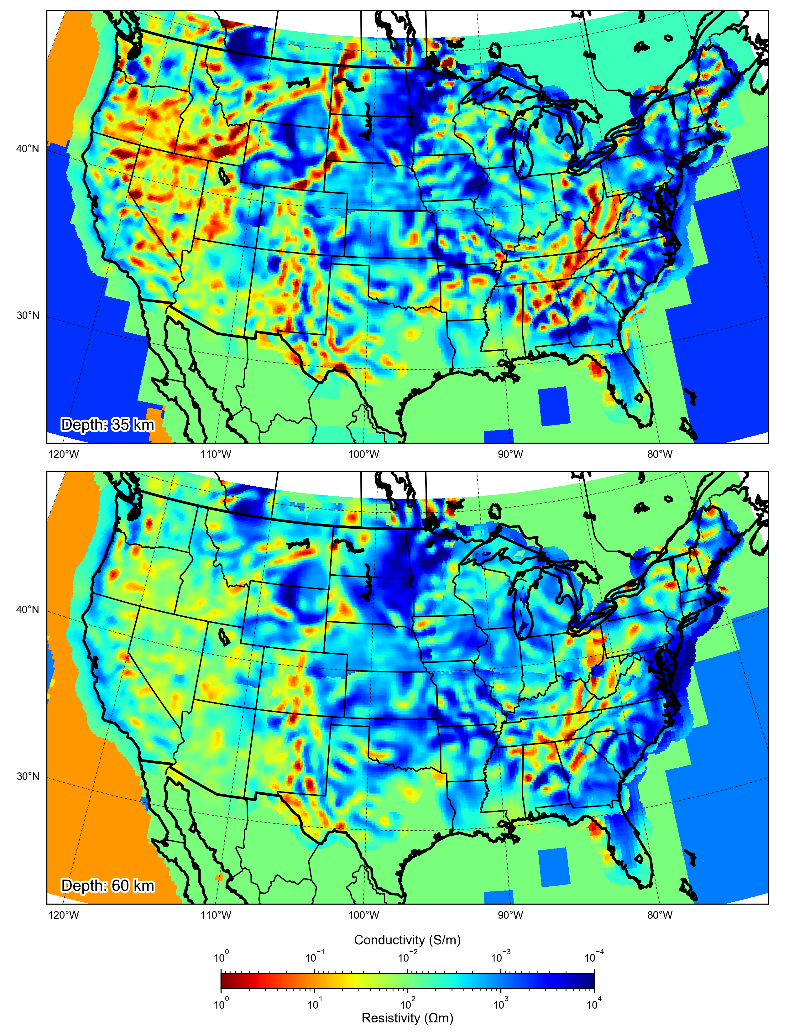
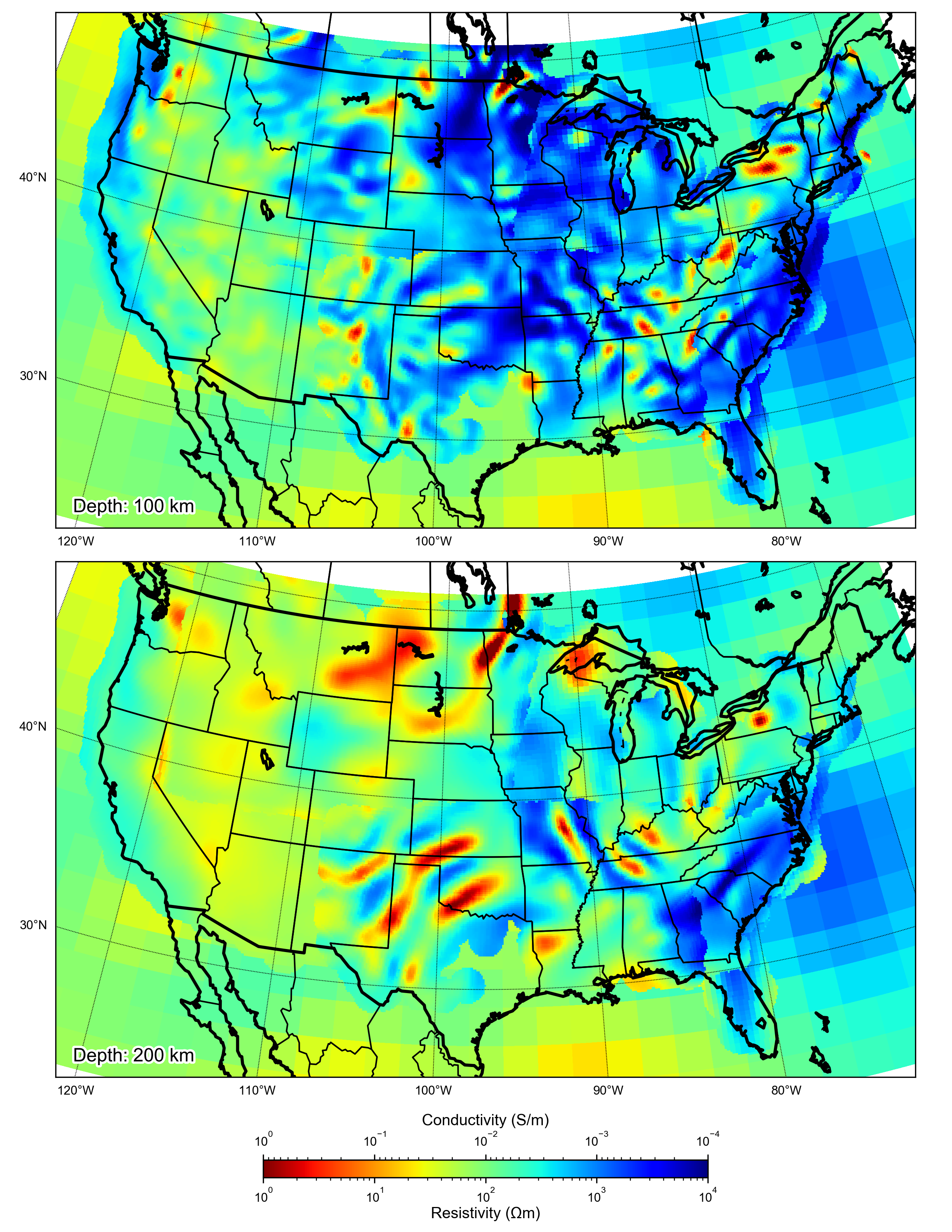
CONUS-MT-2023 is a model of high resolution electrical conductivity variations in the Earth’s crust and mantle of contiguous United States based on magnetotellurics and ground
magnetic observatory data.
Quicklinks
Description
| Name | CONUS-MT-2023 |
| Title | High resolution electrical conductivity variations in the Earth’s crust and mantle of contiguous United States based on magnetotellurics and ground magnetic observatory data. |
| Type | 3-D Continental Electrical Conductivity Model |
| Sub Type | Long-period Magnetotelluric |
| Units | Siemens/meter |
| Year | 2023 |
| Data Revision | r0.0 (revision history) |
| Short Description | To compile the global and regional electrical conductivity models (see References) into a common framework for contiguous United States, which we call CONUS, we created a 3D laterally uniform 0.1° × 0.1° numerical grid. The grid includes the contiguous United States, and extends 650 cells in longitude between −130° and −65°, and 280 cells in latitude between 23° and 51°. Vertically, we started with a 0.1 km top layer, and increased the cell size via a recursive geometric relation with a common ratio of 1.065 until 100 km depth was reached, resulting in 67 vertical layers in the top ∼ 100 km of the grid. Starting at 103.0564 km depth, we extended the grid farther down to ∼ 410 km depth, the top of the mantle transition zone, now starting with a 6.2 km layer and using the same common ratio. This resulted in a total of 90 vertical layers. Finally, we extended the grid from 413.6655 km depth all the way down to 1277 km, using a starting layer of 28 km and the common ratio of 1.07, resulting in a total of 107 Earth layers. We completed the vertical setup by padding the model with four more layers using the common ratio of 1.5, which resulted in the bottom boundary of the model at a 2284.6 km depth. This is done for numerical reasons, so that any inaccuracy in the boundary conditions has minimal effect on the modeling results. Similarly, we also padded the grid laterally by six cells in the North–South directions and seven cells in the East–West directions, to account for the oceans which increase heterogeneity of the model, resulting in a 292 × 664 × 111 numerical grid. For background electrical conductivity in the top 100 km of the Earth’s lithosphere, we used the Alekseev et al. global compilation, modified in the following ways. First, we reduced the background continental resistivity from 5000 Ωm (2 × 10⁻⁴ S/m) to 100 Ωm (10−2 S/m), which is more realistic for average lower crust and uppermost mantle in the contiguous United States. This includes any regions of young oceanic crust, which were left at 100 Ωm background value. We also incorporated the high‐resolution sediment thickness map of Laske and Masters (2015), setting the sediments to a default value of just over 33 Ωm (3 × 10⁻² S/m). Then, this modified model was interpolated to our 0.1° × 0.1° numerical grid with 67 vertical layers in the top 100 km. For background below 100 km depth, the global conductivity model (Sun et al.,) was used. We then proceeded to include MT inverse models, as described in the References, particularly, Kelbert et al. (2019) and Murphy et al. (2023). These models were, first of all, georeferenced from the various Cartesian coordinate projections in which the magnetotelluric inversions have been performed. These selected inverse models and their projection details are further described in these two references. The inverse models were then interpolated to the 0.1° × 0.1° computational grid using the nearest neighbor interpolation, laterally truncated to data locations, and incorporated into the 3D electrical conductivity background in the following order: ENAM, APPL, NEUS, MCR, SWUS, SEUS in the central, then western and eastern United States, followed by EGR and THO. The truncations were defined based on the scale of the model; specifically, models of larger spatial scales and lower resolution (ENAM, MCR, SWUS) were truncated to include structure to within 140 km from a site, equivalent to two times the nominal station spacing of USArray, and WUS was truncated to 105 km (1.5 time station spacing). Other 3D models focused on smaller regions (APPL, NEUS, SEUS, EGR, THO) were truncated to within 70 km from a site, which is equivalent to the nominal station spacing. In the present treatment, no smoothing was applied to model boundaries, to merge the models in places of overlap, other than truncation of all models at a fixed distance from their respective site locations. Thus, the fact that model boundaries generally do not appear as sharp discontinuities speaks to the consistency of these models. In places where models overlap, preferential treatment is given to those models that provide better resolution in the relevant area of the grid (e.g., in the near‐surface) because of magnetotelluric inversion configurations that support higher sensitivity in that area (e.g., shorter periods included in the data set). Relative to CONUS-MT-2021, this model also includes an unpublished inversion result by Benjamin S. Murphy of the USMTArray data in the southcentral U.S. Where well-defined, it overwrites the previous models. Specifically, the new SCUS model is truncated to 105 km (1.5 station spacing) from the nearest station and at depths, to between 1 and 500 km. |
| Authors: | A. Kelbert, Geological Hazards Science Center, Geomagnetism Program, U.S. Geological Survey, Golden, CO, 80401, USA B.S. Murphy, Geological Hazards Science Center, Geomagnetism Program, U.S. Geological Survey, Golden, CO, 80401, USA P. Bedrosian, Geology, Geophysics and Geochemistry Science Center, U.S. Geological Survey, Lakewood, CO, 80215, USA |
| Reference Model | N/A |
| Prior Model | Various (compilation of multiple inverse models) |
| Previous Model | CONUS-MT-2021 |
| Inversion Software | Modular System for Electromagnetic Inversion, Egbert and Kelbert (2012) |
| Model Download | CONUS-MT-2023.r0.0-n4.nc (see metadata) is the above model in netCDF 4 Classic format. |
| Model Homepage | N/A |
| Depth Coverage | 0 – 2,285 km, most reliable to ~250 km depth |
| Area | Focused on the contiguous United States (latitude: 23.1° to 50.9°, longitude: -130.0° to -65.0°) |
| Data Set Description | Frequency domain long-period (10 to 1e4 secs) magnetotelluric (MT) data from USArray MT, USGS MT, USMTArray and other long-period surveys, and multiple wideband (0.01 to 1e3 secs) MT data sets available from IRIS EMTF database (Kelbert, Egbert & Schultz, 2011; http://ds.iris.edu/spud/emtf) |


Citations and DOIs
To cite the original work behind this Earth model:
- Murphy, B.S., Bedrosian, P. and Kelbert, A., 2023. “Geoelectric constraints on the Precambrian assembly and architecture of southern Laurentia”, in Laurentia: Turning Points in the Evolution of a Continent, S.J. Whitmeyer, M.L. Williams, D.A. Kellett and B. Tikoff, Geological Society of America
To cite IRIS DMC Data Products effort:
- Trabant, C., A. R. Hutko, M. Bahavar, R. Karstens, T. Ahern, and R. Aster (2012), Data Products at the IRIS DMC: Stepping Stones for Research and Other Applications, Seismological Research Letters, 83(5), 846–854, https://doi.org/10.1785/0220120032.
DOI for this EMC webpage: https://doi.org/10.17611/dp/emc.2023.conusmt.1
References
- Alekseev, D., A. Kuvshinov, and N. Palshin (2015), Compilation of 3D global conductivity model of the Earth for space weather applications, Earth, Planets and Space, 67(1), 108.
- Bedrosian, P.A. and Finn, C.A., 2021. When Wyoming became Superior: Oblique Convergence along the Southern Trans‐Hudson Orogen. Geophysical Research Letters, https://doi.org/
https://doi.org/10.1029/2021GL092970 .
- Bedrosian, P.A., 2016. Making it and breaking it in the Midwest: Continental assembly and rifting from modeling of EarthScope magnetotelluric data. Precambrian Research, 278, pp.337-361, https://doi.org/
https://doi.org/10.1016/j.precamres.2016.03.009 .
- Egbert G.D. and A. Kelbert. 2012. “Computational recipes for electromagnetic inverse problems.” Geophysical Journal International, 189:251-267, https://doi.org/
https://doi.org/10.1111/j.1365-246X.2011.05347.x .
- Kelbert, A., Bedrosian, P.A. and Murphy, B.S., 2019. The first 3D conductivity model of the contiguous United States: reflections on geologic structure and application to induction hazards. Geomagnetically Induced Currents from the Sun to the Power Grid, pp.127-151, https://doi.org/
https://doi.org/10.1002/9781119434412.ch8
- Kelbert, A., Egbert, G. D. and Schultz, A., 2011. IRIS DMC Data Services Products: EMTF, The Magnetotelluric Transfer Functions. Incorporated Research Institutions for Seismology (IRIS), USA, https://doi.org/
https://doi.org/10.17611/DP/EMTF.1 .
- Laske, G., and G. Masters (1997), A global digital map of sediment thickness, Eos, Transactions, American Geophysical Union, 78(F483), 19–97.
- Meqbel, N.M., Egbert, G.D., Wannamaker, P.E., Kelbert, A. and Schultz, A., 2014. Deep electrical resistivity structure of the northwestern US derived from 3-D inversion of USArray magnetotelluric data. Earth and Planetary Science Letters, 402, pp.290-304, https://doi.org/
https://doi.org/10.1016/j.epsl.2013.12.026 .
- Murphy, B.S. and Egbert, G.D., 2017. Electrical conductivity structure of southeastern North America: Implications for lithospheric architecture and Appalachian topographic rejuvenation. Earth and Planetary Science Letters, 462, pp.66-75, https://doi.org/
https://doi.org/10.1016/j.epsl.2017.01.009 .
- Sun, J., Kelbert, A. and Egbert, G.D., 2015. Ionospheric current source modeling and global geomagnetic induction using ground geomagnetic observatory data. Journal of Geophysical Research: Solid Earth, 120(10), pp.6771-6796, https://doi.org/
https://doi.org/10.1002/2015JB012063 .
Credits
- r0.0 model provided by Anna Kelbert.
Revision History
revision r0.0: uploaded February 14, 2023.
Timeline
- 2023-02-14
- online


