


Summary
Point-source synthetic seismograms are used along with vertical component recordings of short-arc Rayleigh waves (R1) from GCMT Mw7.0+ earthquakes to calculate source-time functions (STF) at GSN and other stations.
Quicklinks
Description
Point-source synthetic seismograms (theoretical Green's functions) are used along with vertical component (LHZ channel) recordings of short-arc Rayleigh waves (R1) from GCMT Mw7.0+ earthquakes to calculate source time functions at GSN and other stations. Source-time functions (STFs) are estimated using a simple two-source forward modeling approach by sweeping through the parameter space of two smoothed triangle and/or trapezoid functions of various widths, offset and amplitude and retaining the best fitting solution.
It is emphasized that this is a fully automated data product with no human review and is intended to serve as a consistent first order baseline. Results should be interpreted keeping this in mind.
Data
For each earthquake, the stations used are determined by initially selecting all available LHZ data between distances of 30-125°. Then the stations are culled to form a set with at least 3° distance between stations with GSN stations taking priority.
Synthetic seismograms
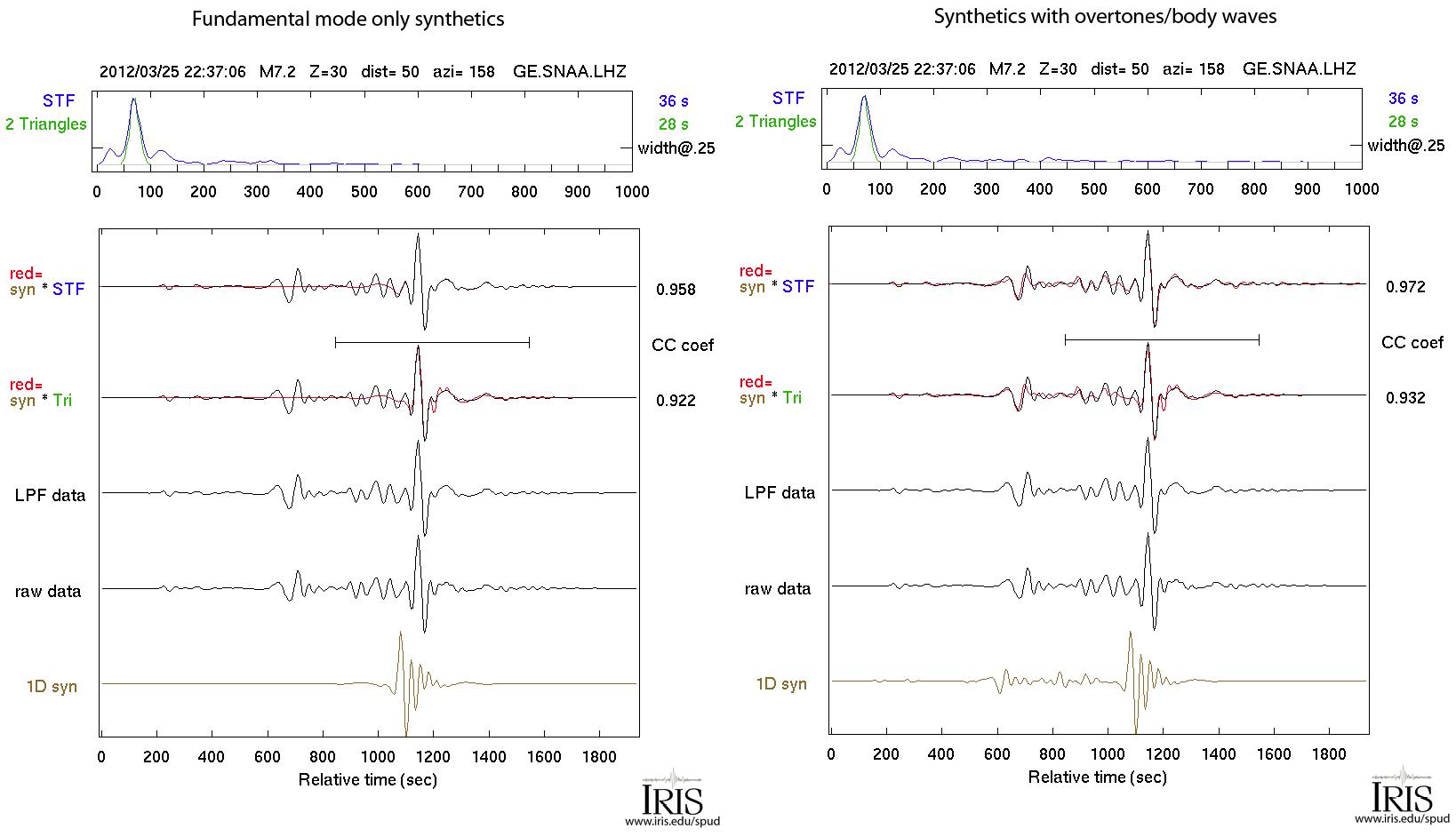
Synthetic seismograms are calculated using normal mode summation (Rivera) using PREM as the reference model and the GCMT solution as the moment tensor. The synthetics are fundamental mode only (no body waves) for simplicity. The R1 signal dominates the waveform in the frequency band examined and results are not significantly different from those that include body waves. Comparison of synthetics with only fundamental modes vs synthetics with overtones/body waves
Preprocessing
-demean, detrend
-deconvolve instrument response to displacement for data. Apply similar filter to synthetics.
-filter:
7.0≤Mag<7.5 0.005 – 0.03 Hz
7.5≤Mag<8.0 0.004 – 0.03 Hz
Mag≥8.0 0.003 – 0.03 Hz
-isolate short-arc Rayleigh waves (R1) using a group-velocity range of 8 km/s to either 2.75 km/s or the start of the major-arc Rayleigh wave (R2) defined by a 5 km/s velocity.
-pad and taper ends with a 300 sec wide Hanning taper
Best fitting 2 source solution STFs
For each point source synthetic seismogram, all combinations of one or two simple sources are explored. Each source permutation is convolved with the synthetic trace, which is then cross-correlated against the data trace over a 700 sec long window around the R1 phase. The combination of sources with the highest cross-correlation coefficient (CCC) is retained. The parameter space includes: one or two sources, variable width sources (triangle shape from 0 – 10 sec half width, trapezoid shape for longer widths up to 120 sec), variable offset between two sources of up to 100 sec, and variable relative amplitude between the two sources.
Iterative time domain deconvolution STFs
The iterative time domain deconvolution approach used is similar to that from Lay (2009), which is adapted from Kikuchi & Kanamori (1982). These supplemental STF results are only included in the .zip attachment of individual station results for completeness and are not plotted in summary figures since the solutions are often complicated and have significant long period noise due to among other things, an imposed positivity constraint. While the waveform fits using this approach tend to match data better (higher CCCs) than the simple 2 source approach, their STFs often contain long period noise and are overly complex. The example with colored traces shown below highlights this. Results from this approach should be interpreted judiciously.
Automated QCing results for summary figures
The preferred solutions for the fully automated R1 RTF solutions presented here reflect the particular parameters chosen for the fully automated data product and should not be considered complete. Results from stations with low cross-correlation coefficients are ignored. Remaining results are binned in either 5 or 15° azimuth windows for figures. Summary figures plot the station result with the highest CCC from each of the windows. Only events with at least 10 different azimuth windows (15° wide each) with results where the highest CCC is at least 0.9 are published in SPUD.
Figures generated for each event

Map with STFs azimuthally plotted
The inset map shows coastlines in solid lines and major tectonic boundaries in dashed lines. Also plotted are the GCMT focal mechanism, and the best fitting STF within 15° wide azimuth bins. For some events, many azimuth bins can be empty due to either no data within the distance (30°-120°) and azimuth range, or the best fitting STF has a CCC below 0.85. A quick glance at this figure indicates wider STFs to the SW and narrower STFs to the NE, consistent with an approximately NE propagating unilateral rupture, implying this event likely ruptured along the NE-striking plane towards the NE. This particular event had a very strong directivity effect; many events in this data product, especially smaller ones with shorter ruptures and deep events, do not show such a clear pattern.
————————————————————————————————————————————————————————————————————

Individual station summary plots (in .zip file)
(Top panel) Example of a station summary figure where the STF from the time-domain deconvolution is in blue and the best fitting simple two-source solution is in green. The width (duration) of the functions at 25% of peak amplitude are given on the right. (Middle panel) The traces shown are the preprocessed (R1 windowed, filtered, response corrected & tapered) synthetic, raw data, and low-pass filtered data used in the deconvolution and a comparison between the data and the estimates formed by convolving the synthetic with either of the STFs. The horizontal bar indicates the range over which the cross-correlation coefficient is calculated. (Lower panel) All station summary figures are bundled in a zip file attachment.
Individual station STFs (as SAC files)
Also in the .zip file are four SAC files for each station analyzed:
-the windowed, filtered and tapered data trace
-the windowed, filtered and tapered synthetic trace
-the STF from the 2 source solution approach
-the STF from the iterative deconvolution approach
Individual station results (as text file)
Also in the attachments is a simple text file of all individual station results which includes the CCCs from both approaches used as well as the duration from the simple 2 source solution approach:

————————————————————————————————————————————————————————————————————

Plots against azimuth
Examples of event summary figures with results aligned by source-to-receiver azimuth. For large unilateral (in one direction) ruptures, an azimuthal pattern emerges where STFs will be compressed at stations in the direction of rupture and longer at stations away from the rupture direction. For events with magnitudes less than about 7.5, results will generally not show much directivity at periods longer than 30 seconds as used in the processing here. In the left figure, the STFs are shaded by their cross-correlation coefficients as described above. The individual station results selected to plot in this figure are based on those with the highest cross-correlation coefficient in 5 degree azimuthal windows. The figure on the right plots all STF widths for results with a CCC > 0.8, with circle size and shading corresponding to the CCC. In both figures, the STF widths appear widest at azimuths around 200° and narrowest at azimuths around 0-60°, consistent with a unilateral rupture towards the NE (azimuths of around 0-60°).
————————————————————————————————————————————————————————————————————


Plots against directivity parameter assuming each of the 2 GCMT strikes
Surface wave phase velocities are close enough to typical earthquake rupture speeds to allow directivity effects to sometimes be observed. For each event the summary figures are also plotted as a function of directivity parameter for each of the two strikes in the GCMT solution. Directivity parameter, Gamma = cos(AziStation – AziStrike)/c, where c is the phase velocity, chosen to be 4.0 km/s, the approximate phase velocity for 30-100 sec period Rayleigh waves. The top panel shows complementary figures with the STFs plotted against Gamma. The bottom panel plots all STF widths for resluts with a CCC > 0.8, lines indicating different rupture velocities (assuming unilateral rupture) for reference, and the average duration, Tavg, in the nomenclature of Lay (2009). Tavg is calculated by a weighted linear regression. See section 3.3 of the reference for further explanation.
————————————————————————————————————————————————————————————————————
Median STF duration
Each summary figure includes a measure of the STF width based on the median width from the best fitting station (cross-correlation coefficient > 0.9) from 5 degree wide azimuthal window bins. The width is measured as the width of the STF between points where amplitudes are >25% of the peak amplitude.
Other Source Time Functions Databases:
- SCARDEC Source Time Functions Database (from teleseismic body waves). The SCARDEC method (Vallée et al., 2011) offers a natural access to the earthquakes source time functions (STFs), together with the 1st order earthquake source parameters (seismic moment, depth and focal mechanism).
Citations and DOIs
To cite the IRIS DMC Data Products effort:
- Hutko, A. R., M. Bahavar, C. Trabant, R. T. Weekly, M. Van Fossen, T. Ahern (2017), Data Products at the IRIS‐DMC: Growth and Usage, Seismological Research Letters, 88, no. 3, https://doi.org/10.1785/0220160190.
To cite the IRIS DMC Source Time Function or reference use of its repository:
- IRIS DMC (2014), Data Services Products: SourceTimeFunction Short-arc Rayleigh wave source-time functions, https://doi.org/10.17611/DP/STF.1.
To reference the use of a particular Source Time Function:
– select the Source Time Function
– click on Citations to obtain its DOI
– insert the DOI in below reference:
- IRIS DMC (2014), Data Services Products: SourceTimeFunction Short-arc Rayleigh wave source-time functions, doi:INSERT DOI HERE.
References
- Lay, T., H. Kanamori, C. J. Ammon, A. R. Hutko, K. Furlong, and L. Rivera (2009), The 2006–2007 Kuril Islands great earthquake sequence, J. Geophys. Res., 114, B11308, https://doi.org/10.1029/2008JB006280.
- Kikuchi, M., and H. Kanamori (1982), Inversion of complex body waves, Bull. Seismol. Soc. Am., 72, 491–506. Link to BSSA
Credits
- Charles Ammon, Penn State University, provided the time domain iterative deconvolution codes.
- Luis Rivera, Universite de Strasbourg, provided the normal mode summation synthetic seismogram codes.
- Alexander Hutko
- IRIS DMC staff implemented and are responsible for the usage and results of the contributed codes.
Timeline
- 2014-03-01
- SourceTimeFunction online


