Summary
Visualizations of real data showing how seismic waves from earthquakes sweep across the North American network of seismic stations for which data are openly available and are collected using the federated data access.
Quicklinks
- View GMVs
- Super (combined) GMVs
- GMV Python 3 code (GitHub)
- Citations
Description

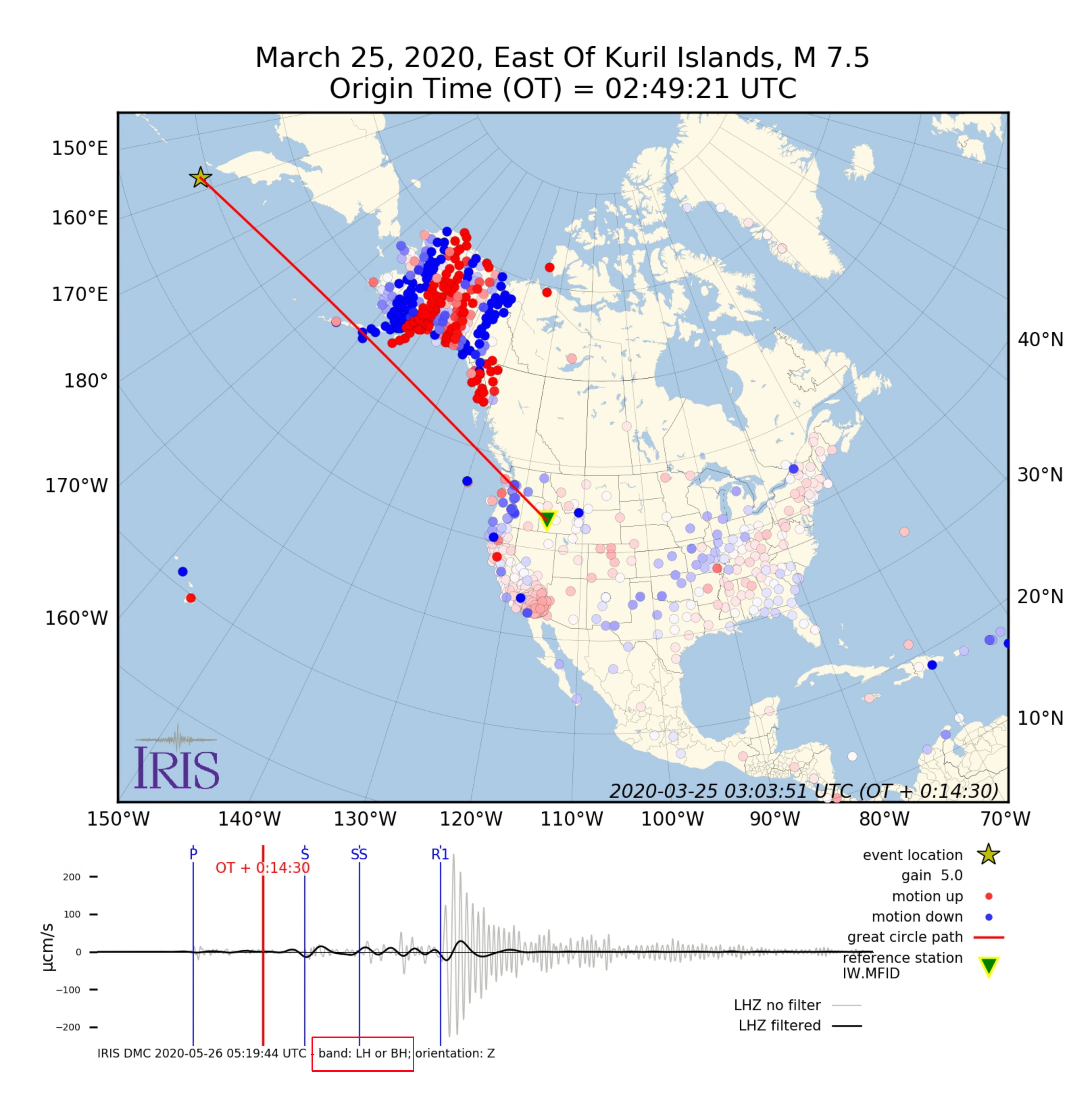
The Ground Motion Visualization (GMV) is a video-based IRIS DMC data product that illustrates how seismic waves travel away from an earthquake location by animating the normalized recorded wave amplitudes at each seismometer location using colored markers. Color of each marker depicts amplitude of the vertical ground motion, as detected by the station’s seismometer and normalized to its peak amplitude. The color changes as waves of differing amplitude travel past the seismometer. Blue • indicates downward ground motion while red • represents upward ground motion with the darker colors indicating larger ground motions (Figure 1).
GMVs were originally produced using a MATLAB script that utilized the Long period, High gain data, with different channel orientations (LH? channel data) from the Transportable Array (TA) component of the USArray/EarthScope project and its Backbone stations. On December 6, 2017 pool of the contributing stations was expanded to include the “realtime” LH? data from all North American stations available through DMC (_REALTIME virtual network).

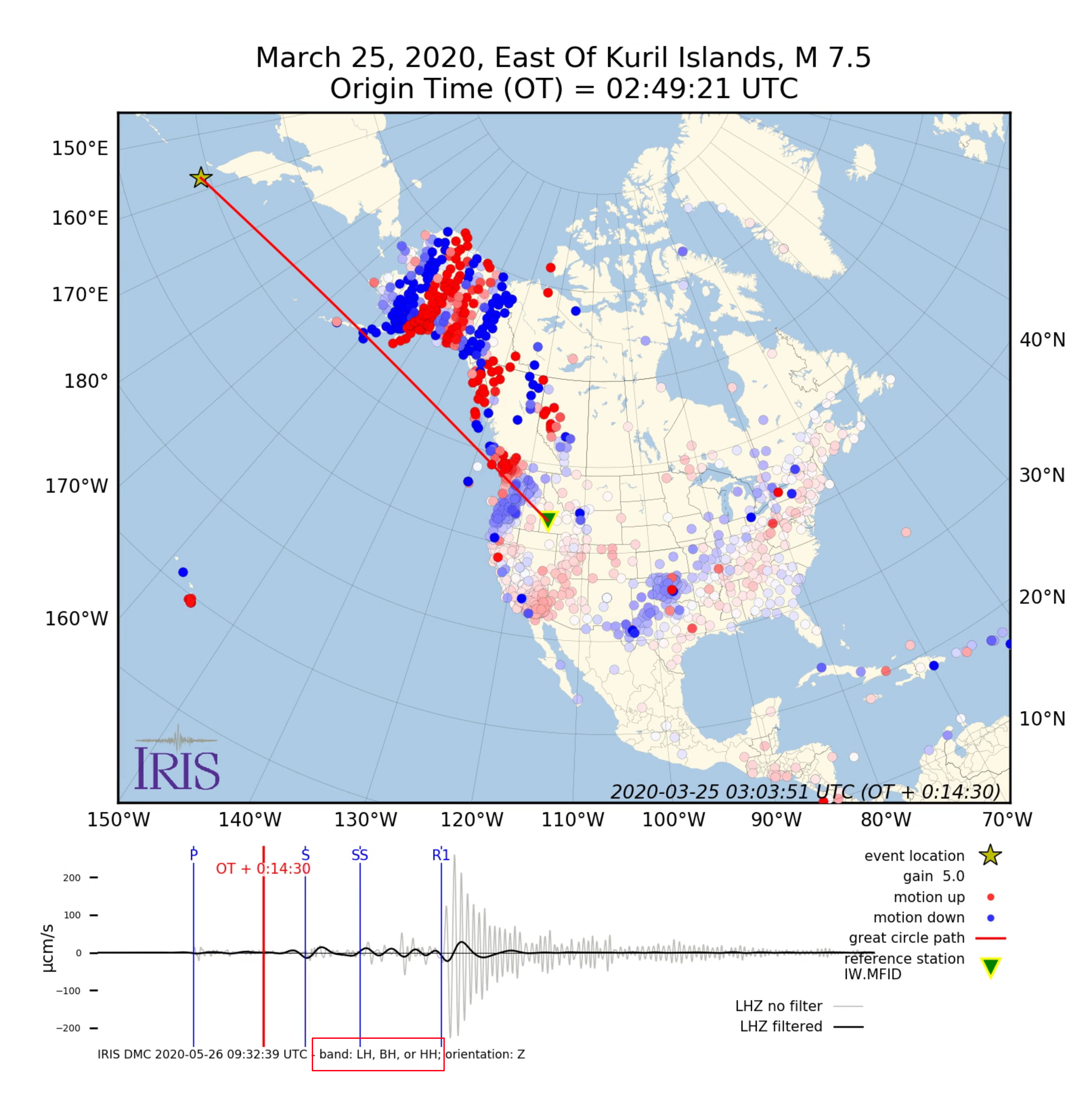
Starting June 1, 2020, GMVs are produced by a Python code that uses all available open waveform data through the federated data access. This federated system allows retrieval of available open data from seismic stations across multiple FDSN Data Centers. To publish GMVs in a timely fashion, GMVs are created and distributed in two steps. In the first pass, GMVs are created using LH? or BH? channel data from all available stations and are labeled accordingly (label highlighted by a red rectangle in Figure 2). To create these GMVs, all waveform data are corrected for the instrument response and then each seismogram is independently normalized to its maximum amplitude. About two hours after publishing the first set of GMVs, the “final” GMVs, usually with a better station coverage, go into production using data from LHZ, BHZ, or HHZ channels (Figure 3).
To highlight weaker arrivals, at the expense of saturating colors of the stronger arrivals, a constant gain is applied to all input traces. GMV’s default gain is 5 and it is suitable for most events. However, for the events closer to the viewport (between 10°- 20° from the viewport’s center), the gain is dropped to 4 and for even closer events (less than 10 degrees from the viewport’s center), the gain is set to 3. This change in magnification prevents extreme highlighting of the unwanted near-source arrivals. To reduce the effect of noisy stations, a standard deviation analysis is performed on the first 5 minutes of each trace and traces that exhibit high standard deviation are rejected.
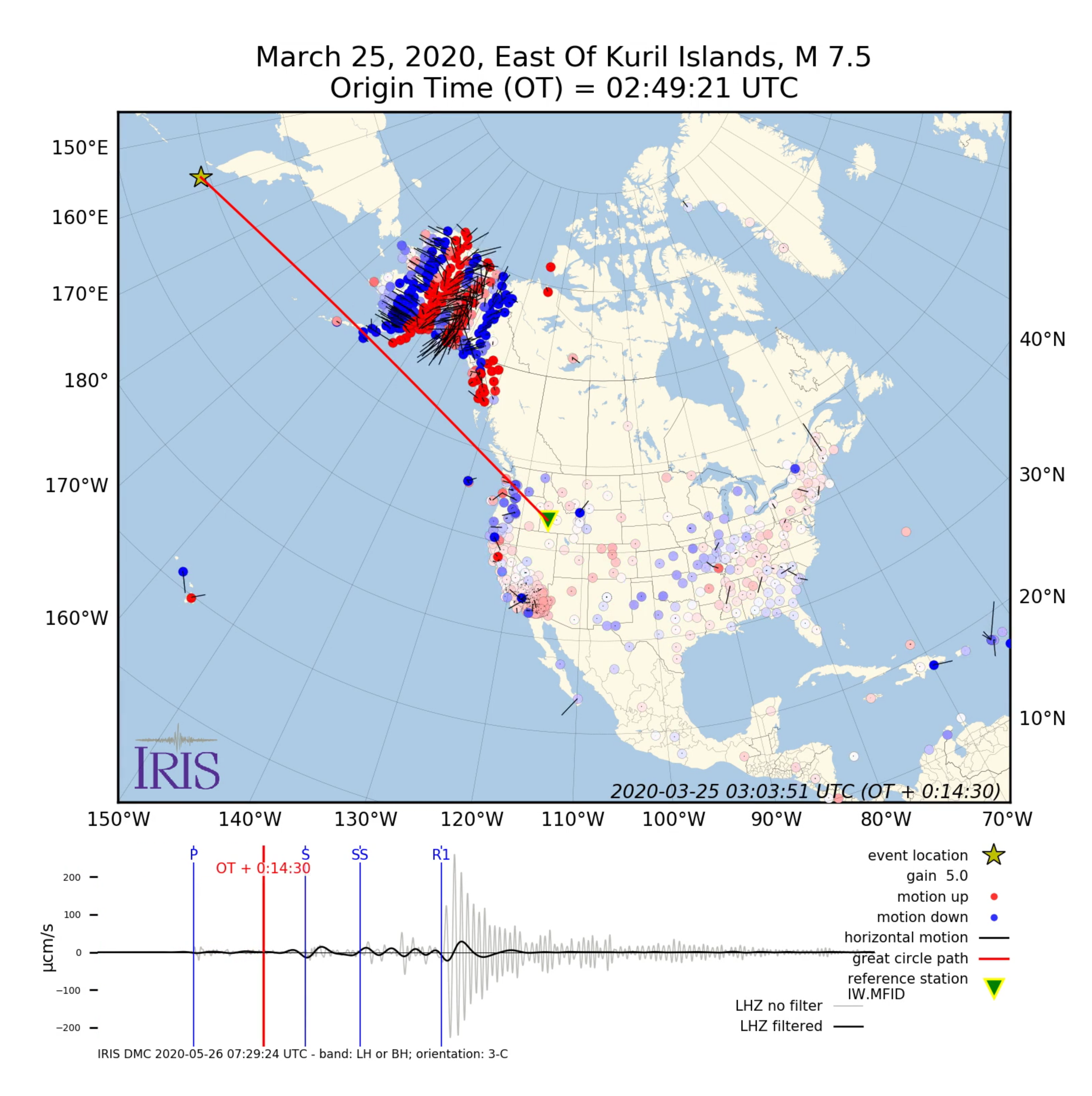
For large events, magnitude ≥ 7, in addition to the vertical component GMVs (Figure 3), 3-component GMVs (Figure 4) are also produced that incorporate plot of the vector field (quiver) with direction and length of their tails representing direction and amplitude of the normalized horizontal ground motion respectively. For the 3-component GMVs, the horizontal traces are normalized together. Table 1 provides a summary of parameters used to create GMVs.
Table 1: A summary of parameters used to generate GMVs.
| PARAMETER | vertical-component | 3-component |
|---|---|---|
| Network | all from FDSN | all from FDSN |
| Channel | Initial set: LHZ or BHZ Final set: LHZ, BHZ, or HHZ |
LH? or BH? |
| Event magnitude (M) | US: M ≥ 5.5 world: M ≥ 6 |
M ≥ 7 |
| Instrument response | removed (output as velocity) | removed (output as velocity) |
| Filter band base on event magnitude (M) | 6.0 > M ≥ 5.5: 0.02 Hz – 0.05 Hz 6.5 > M ≥ 6.0: 0.004 Hz – 0.02 Hz M ≥ 6.5: 0.002 Hz – 0.01 |
M ≥ 7: 0.002 Hz – 0.01 Hz |
| Travel-time estimation | iasp91 Earth model | iasp91 Earth model |
| Rayleigh slowness | 28.5 s/degree | 28.5 s/degree |
To compliment the ground motion visualizations and to provide a sense for the ground displacement, a representative vertical seismogram from an arbitrary station (reference station) is also plotted under each GMV animation. The location of this reference station is marked by a down-pointing green triangle ▼ on the map. The horizontal axis of this plot represents time after the origin time (OT), and a moving vertical red line shows time on the seismogram corresponding to the displayed GMV frame.
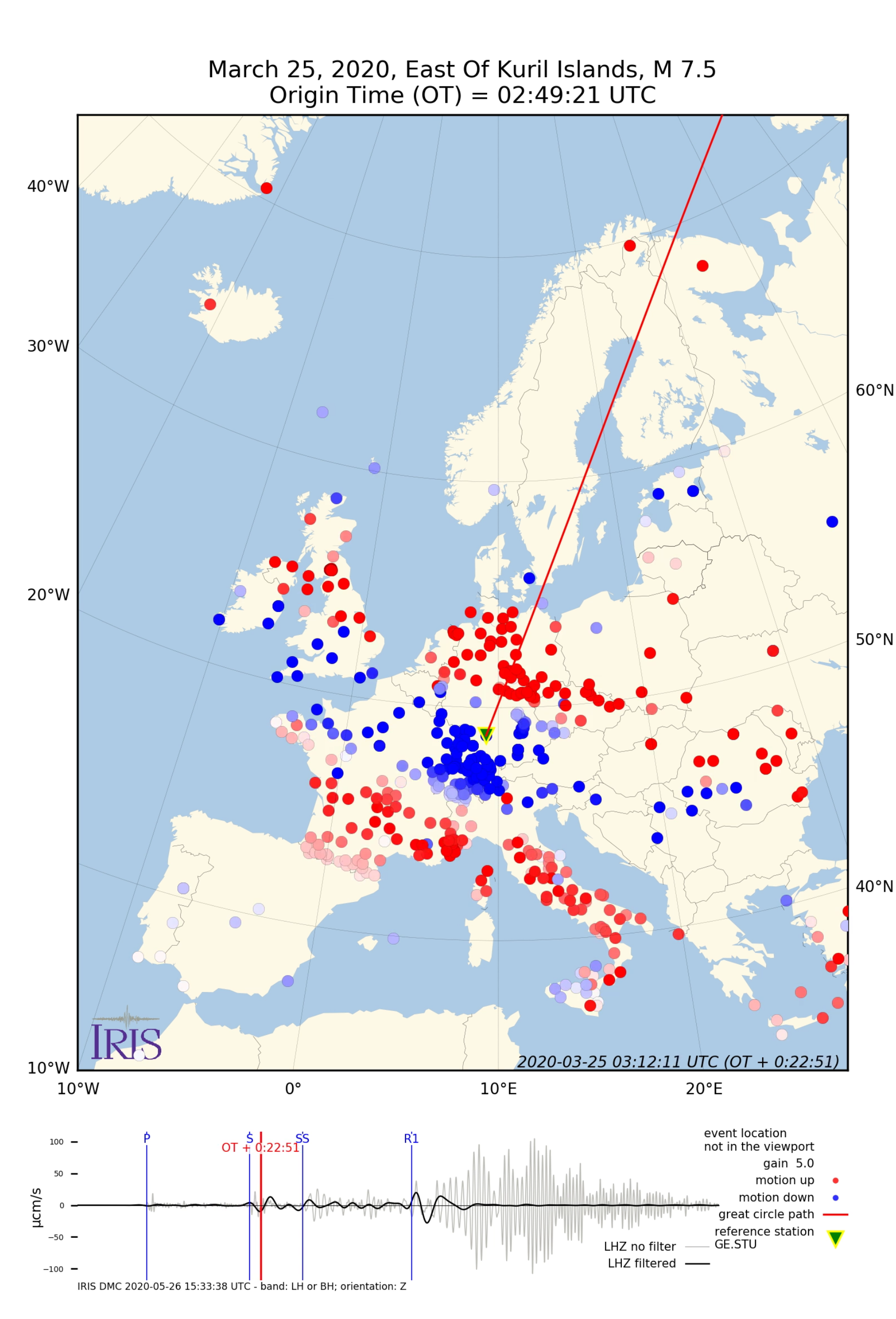
Under favorable conditions, but not as part of the automated GMV production, it is possible to point GMV production to a different viewport (Figure 5), or to combine GMVs from “repeated” sources to create a Super (Combined) GMV.


Citations and DOIs
To cite the IRIS DMC Data Products effort:
- Trabant, C., A. R. Hutko, M. Bahavar, R. Karstens, T. Ahern, and R. Aster (2012), Data Products at the IRIS DMC: Stepping Stones for Research and Other Applications, Seismological Research Letters, 83(5), 846–854, https://doi.org/10.1785/0220120032.
To cite the IRIS DMC GMV data product or reference use of its repository:
- IRIS DMC (2010), Data Services Products: GMV, The Ground Motion Visualization, https://doi.org/10.17611/ds/gmv.1
To cite the source or reference the use of a particular GMV:
– select the GMV of interest
– click on Citations to obtain its DOI
– insert the DOI in below reference:
- IRIS DMC (2010), Data Services Products: GMV The Ground Motion Visualization, doi:INSERT DOI HERE.
Credits
- Chuck Ammon, Professor of Geosciences at Penn State’s original concept and visualizations.
- Bob Woodward at IRIS – adapted the visualization code to MATLAB
- Manochehr Bahavar, IRIS DMC
Timeline
- 2010-02-25
- GMV online, automated production of GMV started
- 2010-10-20
- 3-component GMVs online
- 2011-03-24
- Customized GMV online
- 2013-10-22
- Super GMVs online
- 2015-10-05
- Expanded to include Alaska
- 2020-06-01
- Installed Generalized GMV 1.0


