Earth models are often defined on a geographic grid that follow lines of constant latitude and longitude. However, for some models, a projected coordinate system, such as UTM, is preferred because it results in less local distortion.

In 2010, when the netCDF file format was first adopted by EMC, the targeted models were often expressed in the geographic coordinate system, and therefore, the EMC’s netCDF format definition included the coordinate variables latitude and longitude (Table 1, left), 2D model variables (e.g., thickness) with latitude and longitude dimensions, and the 3D variables (e.g., velocity) with latitude, longitude, and depth dimensions. As the number of models expressed in projected coordinate systems is increasing, the EMC’s netCDF format is extended to support such models.

The extended EMC netCDF format includes both the projected coordinate system variables (x and y) and the geographic latitude and longitude variables that are defined as a function of the primary x and y coordinate variables (Table 1, right). These two-dimensional latitude and longitude coordinate variables allow users to quickly switch between the model’s projected coordinates and the geographic latitudes and longitudes. In this extended netCDF format, the x and y of the projection coordinate system become the primary coordinates, and the geographic latitude and longitude, which depend on x and y, represent the auxiliary coordinate variables. The directions of the primary coordinate variables are defined by adding the axis attribute to the x and y coordinate variables. The model variables (thickness and vp in Table 1, right) are now defined based on the primary x and y coordinate variables, and are tied to the auxiliary coordinate variables via the coordinates attribute.

Table 1. A comparison of dimensions and variables in a classic EMC model with geographic coordinates (left), and in an extended EMC model with a projected coordinate system (right).

Data extraction and grid mapping

In the following simple Python 3 code snippets, we use the xarray to demonstrate that data from model files with two-dimensional latitude and longitude are accessible using either the coordinate indices, the primary coordinates, or the geographic coordinates. In these examples, we access the shear velocity (vs) data from the nz-atom-north-chow-etal-2021-vp+vs-crust.r0.0-n4.nc (metadata) file of the New Zealand Adjoint TOMography velocity model by Chow et al. (2022).

First, open and decode an xarray dataset (ds) from the netCDF file for the desired variable (vs in this example):

import numpy as np
import xarray as xr
# 
fname = "nz-atom-north-chow-etal-2021-vp+vs-crust.r0.0-n4.nc"
varname = "vs"
# 
ds = xr.open_dataset(fname)
dsv = ds[varname]

i, j, k = 21,75,3
ds2 = dsv.isel(x=i, y=j, depth=k)
#
print(f"\n\ni={i}, j={j}, k={k}\ndepth\ty\tx\tlatitude\tlongitude\tvs\n"
      f"{ds2.depth.values}\t{ds2.y.values}\t{ds2.x.values}\t"
      f"{ds2.latitude.values:0.3f}\t\t{ds2.longitude.values:0.3f}\t\t{ds2.values:0.3f}\n"))

To access the same grid point but via x, y, and depth values, use the xarray.DataArray.where filter and then convert the filtered dataset to a dataframe and remove the “nan” values that represent the values that were masked by the where filter:

x, y, depth = 191.0, 5361.0, 8.5
print(f"\n\nx={x}, y={y}, depth={depth}")
#
ds2 = dsv.where((dsv.x = = x) & (dsv.y = = y) & (dsv.depth == depth))
#
df = ds2.to_dataframe()
df.dropna(inplace=True)
print(df)

And finally, we could query the dataset based on the latitude, longitude and depth values above:

latitude, longitude, depth = -41.842999, 173.278, 8.5
print(f"\n\nlongitude={longitude}, latitude={latitude}, depth={depth}")
#
ds2 = dsv.where((dsv.longitude = = longitude) & (dsv.latitude = = latitude) & (dsv.depth == depth))
#
df = ds2.to_dataframe()
df.dropna(inplace=True)
print(df)

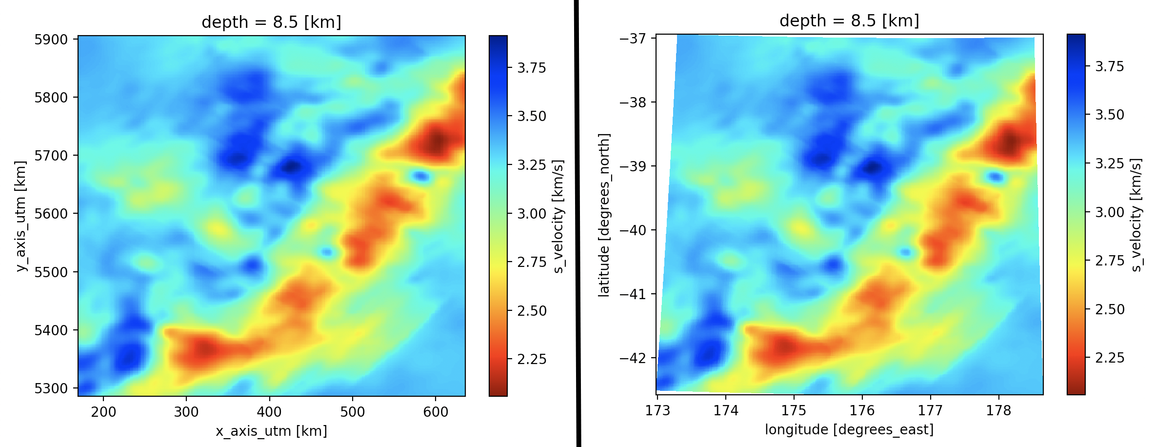
We can also switch between coordinate systems when plotting a horizontal slice of this dataset at the above depth (index 3 at 8.5 km). By default, the plot will be in the primary coordinate system of the model (UTM, Figure 1, left). To create a plot based on the geographic coordinates, in the below code snippet, we explicitly reference the auxiliary latitude and longitude coordinates (Figure 1, right):

import matplotlib.pyplot as plt
#
# Plot with the primary coordinates in UTM (Figure 1, left).
ds.vs[3].plot(cmap='jet_r')
plt.show()
#
# Use the auxiliary coordinates (latitude, longitude) to plot (Figure 1, right).
ds.vs[3].plot(x="longitude", y="latitude", cmap='jet_r')
plt.show()

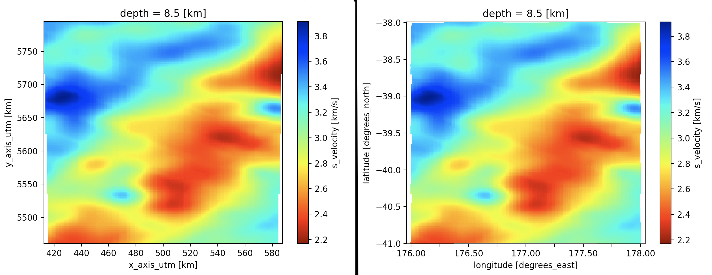
Finally, the following snippet uses the where function to limit the slice in Figure 1 to the area bounded between 176° to 178° longitude and -41° to -38° latitude. Again, by default, the corresponding plot will be in the primary coordinate system of the model (UTM, Figure 2, left). To create a plot based on the geographic coordinates, we need explicitly reference the auxiliary coordinates (Figure 2, right):

# Subset the data.
#
lon_min, lon_max = 176.0, 178.0
lat_min, lat_max = -41.0, -38.0
depth = 8.5
ds_selected = dsv.where((dsv.longitude >= lon_min) & (dsv.longitude <= lon_max) &
                        (dsv.latitude >= lat_min) & (dsv.latitude <= lat_max) &
                        (dsv.depth == depth), drop=True)
#
# Plot with the primary coordinates in UTM (Figure 2, left).
ds_selected.plot(cmap='jet_r')
plt.show()
#
# Use the auxiliary coordinates (latitude, longitude) to plot (Figure 2, right).
ds_selected.plot(x="longitude", y="latitude", cmap='jet_r')
plt.show()

Links

IRIS Earth Model Collaboration

How to contribute Earth models to EMC

EMC Tools

Climate and Forecast (CF) Metadata Conventions