Summary
CAM2016, Priestley et al. (2016), is a group of global upper models based on multi-mode surface wave tomography.
Quicklinks
Description
| Name | CAM2016 |
| Title | Global upper mantle surface wave tomography model |
| Type | 3-D Tomography Earth Model |
| Sub Type | S velocity |
| Year | 2016 |
| Short Description | CAM2016 is a group of global upper mantle models based on multi-mode surface wave tomography. Details of the analysis procedures are given in Cara & Leveque (1987), Debayle & Sambridge (2004), Priestley et al (2006), Debayle & Ricard (2012), Priestley & McKenzie (2013) and Ho et al (2016). These models include an upper mantle Vsv model CAM2016Vsv derived from the waveform modeling of more than 2 million vertical component Rayleigh waveforms, an upper mantle Vsh model CAM2016Vsh from the waveform modeling of ~0.5 million transverse component Love waveforms, a radial anisotropic model CAM2016Xi derived from the waveform modeling of ~0.25 million Rayleigh and Love waveforms with common propagation paths, a lithospheric thickness model CAM2016Litho, and an upper mantle thermal model CAM2016T-200. All models are defined on a 2 degree by 2 degree grid. Vsv and Vsh models are given for several lateral smoothing lengths. The models determined with the shorter smoothing length are applicable to the shallower depths while the models determined with the larger smoothing length are more appropriate to the deeper depths. |
| Authors: | |
| Keith Priestley | |
| Bullard Laboratories | |
| Department of Earth Sciences | |
| University of Cambridge | |
| Cambridge, United Kingdom | |
| Tak Ho | |
| Bullard Laboratories | |
| Department of Earth Sciences | |
| University of Cambridge | |
| Cambridge, United Kingdom | |
| Previous Model | |
| Reference Model | SPREM |
| Model Homepage | https://www.esc.cam.ac.uk/directory/keith-priestley |
| Model Download | |
Each of the following compressed TAR Archive files contains separated files for each depth of upper mantle model CAM2016:
|
|
| CAM2016Vsv_200.tgz CAM2016Vsv_400.tgz CAM2016Vsv_600.tgz CAM2016Vsv_800.tgz CAM2016Vsh_400.tgz CAM2016Vsh_600.tgz CAM2016Vsh_800.tgz CAM2016Xi-400.tgz CAM2016Xi-600.tgz CAM2016Xi-800.tgz CAM2016T-200.tgz CAM2016Litho.tgz |
|
CAM2016Litho.nc (see metadata ), is the netCDF file for the model |
|
| CAM2016T-200.nc (see metadata ), is the netCDF file for the upper mantle T model CAM2016Vsh-400.nc (see metadata ), is the netCDF file for the thickness (km) of the thermal lithosphere CAM2016Vsh-600.nc (see metadata ), is the netCDF file for the model CAM2016Vsh-800.nc (see metadata ), is the netCDF file for the model CAM2016Vsv-200.nc (see metadata ), is the netCDF file for the model CAM2016Vsv-400.nc (see metadata ), is the netCDF file for the model CAM2016Vsv-600.nc (see metadata ), is the netCDF file for the model CAM2016Vsv-800.nc (see metadata ), is the netCDF file for the model CAM2016Xi-400.nc (see metadata ), is the netCDF file for the model CAM2016Xi-600.nc (see metadata ), is the netCDF file for the model CAM2016Xi-800.nc (see metadata ), is the netCDF file for the model |
|
| Depth Coverage | Upper mantle (40 to 680 km) |
| Area | Global |
| Data Set Description | Models are derived from all waveforms with CMT solutions currently available at the IRIS and EIDA data centers plus additional waveform data for Southern Asia. All models defined on a 2 degree by 2 degree grid. Vsv models are provided for four smoothing lengths; Vsh models are provided for three smoothing lengths. For wave-speed models the absolute shear wave speed, the perturbation to the layer average, and perturbation to the reference model are tabulated. |

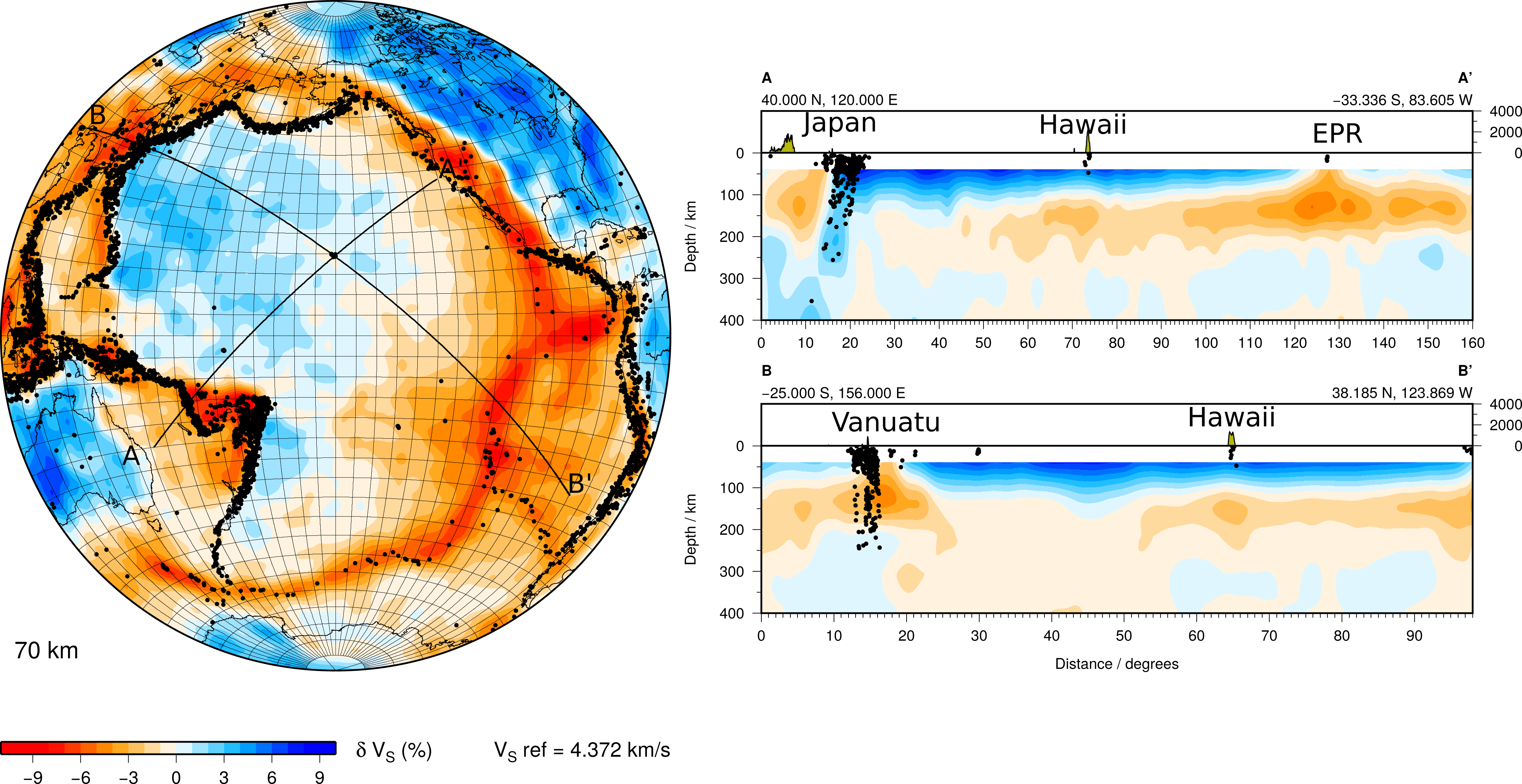
wave-speed with respect to the reference model at 70 km depth for the Pacific
hemisphere. The scale at left beneath the map shows the percent perturbation
at this depth with respect to the reference wave-speed (SPREM_Vsv) at this
depth whose value (Vsref) is shown below the map at right. The lateral smoothing
half-width is 200 km. The two lines on the map marked AA’ and BB’ show the
locations of the two cross-sections shown at right in the figure.

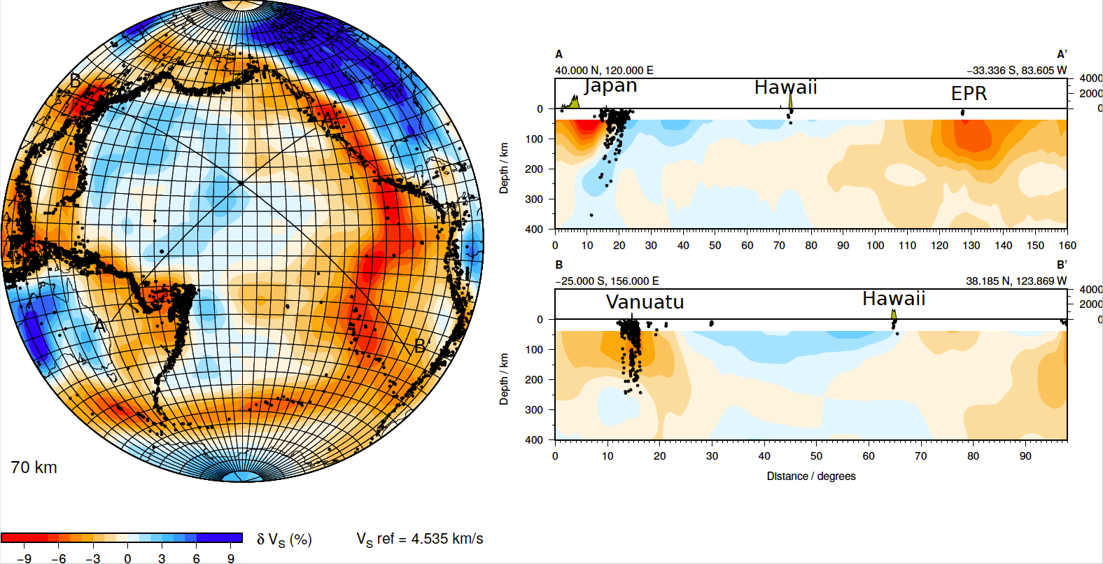
wave-speed with respect to the reference model at 70 km depth for the Pacific
hemisphere. The scale at left beneath the map shows the percent perturbation
at this depth with respect to the reference wave-speed (SPREM_Vsh) at this
depth whose value (Vsref) is shown below the map at right. The lateral
smoothinghalf-width is 600 km. The two lines on the map marked AA’ and BB’
show the locations of the two cross-sections shown at right in the figure.

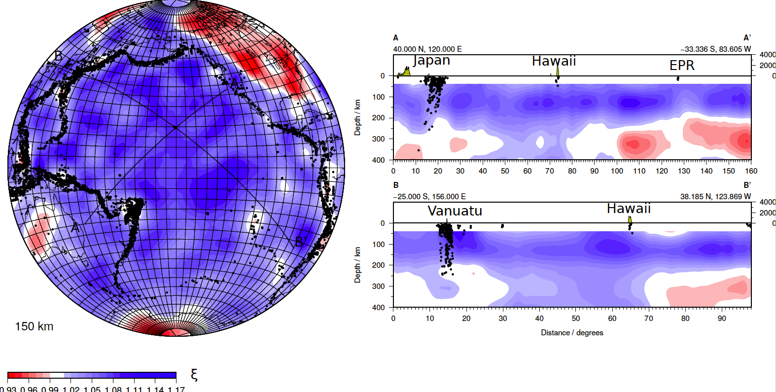
depth for the Pacific hemisphere. The scale at left beneath the map shows the
magnitude of the radial anisotropy. The two lines on the map marked AA’ and BB’
show the locations of the two radial anisotropy cross-sections shown at right in
the figure.

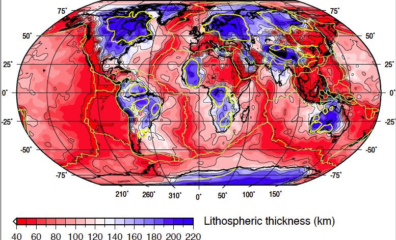
model CAM2016Vsv. The lithospheric model was derived by converting the Vsv
model to a temperature model using the Vs(T) relationship described in
(Priestley & McKenzie, 2013), then examining the geotherm at each geographic
point of the model and identifying the depth of the transition from the
conducting to advecting geotherm. The yellow contour denotes the
geologically-mapped boundary of the shields at the surface.
Citations and DOIs
To cite the original work behind this Earth model:
- Ho, T., K. Priestley, and E. Debayle (2016), A global horizontal shear velocity model of the upper mantle from multimode Love wave measurements, Geophysical Journal International, 207(1), 542–561. https://doi.org/10.1093/gji/ggw292
- Priestley, K., and D. McKenzie (2013), The relationship between shear wave velocity, temperature, attenuation and viscosity in the shallow part of the mantle, Earth and Planetary Science Letters, 381, 78–91. https://doi.org/10.1016/j.epsl.2013.08.022
- Priestley, K. , McKenzie, D. and Ho, T. (2019). A Lithosphere–Asthenosphere Boundary—a Global Model Derived from Multimode Surface‐Wave Tomography and Petrology. In Lithospheric Discontinuities (eds H. Yuan and B. Romanowicz). https://doi.org/10.1002/9781119249740.ch6
To cite IRIS DMC Data Products effort:
- Trabant, C., A. R. Hutko, M. Bahavar, R. Karstens, T. Ahern, and R. Aster (2012), Data Products at the IRIS DMC: Stepping Stones for Research and Other Applications, Seismological Research Letters, 83(5), 846–854, https://doi.org/10.1785/0220120032.
DOI for this EMC webpage:
References:
Cara, M., and J. Leveque (1987), Waveform inversion using secondary observables, Geophysical Research Letters, 14(10), 1046–1049.
Debayle, E., and M. Sambridge (2004), Inversion of massive surface wave data sets: model construction and resolution assessment, Journal of Geophysical Research: Solid Earth, 109(B2).
Debayle, E., and Y. Ricard (2012), A global shear velocity model of the upper mantle from fundamental and higher Rayleigh mode measurements, Journal of Geophysical Research: Solid Earth, 117(B10).
Priestley, K., and D. McKenzie (2006), The thermal structure of the lithosphere from shear wave velocities, Earth and Planetary Science Letters, 244(1), 285–301.
Credits
Model provided by Keith Priestley
Timeline
- 2018-05-11
- online
- 2021-07-01
- added CAM2016Xi-400 and CAM2016Xi-800 model files


